最も単純そうなDataSourceプラグインを読んでいく。
プラグインは simpod-json-datasource plugin。
配布はここ。
JSONを返す任意のURLにリクエストを投げて結果を利用できるようにする。
TypeScriptで書かれている。
The JSON Datasource executes JSON requests against arbitrary backends.
JSON Datasource is built on top of the Simple JSON Datasource. It has refactored code, additional features and active development.
install
インストール方法は以下の通り。
初回だけgrafana-serverのrestartが必要。
# install plugin
$ grafana-cli plugins install simpod-json-datasource
# restart grafana-server
$ sudo service grafana-server restart
build
ビルド方法は以下の通り。
yarn一発。
# build
$ cd /var/lib/grafana/plugins/simpod-json-datasource
$ yarn install
$ yarn run build
設定
データソースの追加で、今回インストールした DataSource/JSON (simpod-json-datasource)を
選択すると、プラグインのコンフィグを変更できる。
要求するURL一覧
URLはBaseURL。
このプラグインはURLの下にいくつかのURLが存在することを想定している。
つまり、それぞれのURLに必要な機能を実装することでプラグインが機能する。
用語については順に解説する。
必須
Method
Path
Memo
GET
/
ConfigページでStatusCheckを行うためのURL。200が返ればConfigページで「正常」となる。
POST
/search
呼び出し時に「利用可能なメトリクス」を返す。
POST
/query
「メトリクスに基づくデータポイント」を返す。
POST
/annotations
「アノテーション」を返す。
オプショナル
Method
Path
Memo
POST
/tag-keys
「ad-hocフィルタ」用のタグのキーを返す。
POST
/tag-values
「ad-hocフィルタ」用のタグの値を返す。
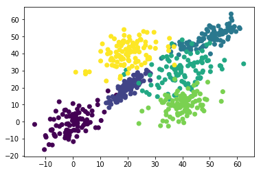
メトリクス
Grafanaにおいて、整理されていないデータの中から\"ある観点\"に従ったデータを取得したいという
ユースケースをモデル化している.
例えば、サーバ群の負荷状況を監視したいというケースでは「サーバ名」毎にデータを取得したいし、
センサ群から得られるデータを監視したいというケースでは「センサID」毎にデータを取得したい.
これらの観点は、Grafanaにおいて「メトリクス」または「タグ」として扱われる。
センサAからセンサZのうちセンサPとセンサQのデータのみ表示したい、という感じで使う。
ここで現れるセンサAからセンサZが「メトリクス」である。
クエリ変数のサポート (metricFindQuery)
「クエリ変数」は、「メトリクス」を格納する変数である。
データソースプラグインがクエリ変数をサポートするためには、
DataSourceApi クラスの metricFindQuery を オーバーライド する.
string型のqueryパラメタを受け取り、MetricFindValue型変数の配列を返す.
要は以下の問答を定義するものである。
- 質問 : 「どんなメトリクスがありますか?」
- 回答 : 「存在するメトリクスはxxx,yyy,zzzです」
ちなみに、metricFindQueryが受け取るqueryの型は、
metricFindQueryを呼び出すUIがstring型で呼び出すからstring型なのであって、
UIを変更することで別の型に変更することができる。
以下、simpod-json-datasource の metricFindQuery の実装。
// MetricFindValue interfaceはtext,valueプロパティを持つ
// { \"label\":\"upper_25\", \"value\": 1}, { \"label\":\"upper_50\", \"value\": 2} のような配列を返す.
metricFindQuery(query: string, options?: any, type?: string): Promise {
// Grafanaが用意する interpolation(補間)関数
// query として \"query field value\" が渡されたとする
// interpolated は { \"target\": \"query field value\" }のようになる.
const interpolated = {
type,
target: getTemplateSrv().replace(query, undefined, \'regex\'),
};
return this.doRequest({
url: `${this.url}/search`,
data: interpolated,
method: \'POST\',
}).then(this.mapToTextValue);
}
// /searchから返ったJSONは2パターンある
// 配列 ([\"upper_25\",\"upper_50\",\"upper_75\",\"upper_90\",\"upper_95\"])か、
// map ([ { \"text\": \"upper_25\", \"value\": 1}, { \"text\": \"upper_75\", \"value\": 2} ])
// これらを MetricFindValue型に変換する
mapToTextValue(result: any) {
return result.data.map((d: any, i: any) => {
// mapの場合
if (d && d.text && d.value) {
return { text: d.text, value: d.value };
}
// 配列の場合
if (isObject(d)) {
return { text: d, value: i };
}
return { text: d, value: d };
});
}
以下、simpod-json-datasource が メトリクスを取得する部分のUI。
FormatAs, Metric, Additional JSON Dataの各項目が選択可能で、
各々の変数がViewModelとバインドされている.
コードは以下。React。
FormatAsのセレクトボックスのOnChangeでsetFormatAs()が呼ばれる。
MetricのセレクトボックスのOnChagneでsetMetric()が呼ばれる。
Additional JSON DataのonBlurでsetData()が呼ばれる。
import { QueryEditorProps, SelectableValue } from \'@grafana/data\';
import { AsyncSelect, CodeEditor, Label, Select } from \'@grafana/ui\';
import { find } from \'lodash\';
import React, { ComponentType } from \'react\';
import { DataSource } from \'./DataSource\';
import { Format } from \'./format\';
import { GenericOptions, GrafanaQuery } from \'./types\';
type Props = QueryEditorProps;
const formatAsOptions = [
{ label: \'Time series\', value: Format.Timeseries },
{ label: \'Table\', value: Format.Table },
];
export const QueryEditor: ComponentType = ({ datasource, onChange, onRunQuery, query }) => {
const [formatAs, setFormatAs] = React.useState<selectableValue>(
find(formatAsOptions, option => option.value === query.type) ?? formatAsOptions[0]
);
const [metric, setMetric] = React.useState<selectableValue>();
const [data, setData] = React.useState(query.data ?? \'\');
// 第2引数は依存する値の配列 (data, formatAs, metric).
// 第2引数の値が変わるたびに第1引数の関数が実行される.
React.useEffect(() => {
// formatAs.value が 空なら何もしない
if (formatAs.value === undefined) {
return;
}
// metric.value が 空なら何もしない
if (metric?.value === undefined) {
return;
}
// onChange(..)を実行する
onChange({ ...query, data: data, target: metric.value, type: formatAs.value });
onRunQuery();
}, [data, formatAs, metric]);
// Metricを表示するセレクトボックスの値に関数がバインドされている.
// 関数はstring型のパラメタを1個とる.
const loadMetrics = (searchQuery: string) => {
// datasourceオブジェクトの metricFindQuery()を呼び出す.
// 引数はsearchQuery. 戻り値はMetricFindValue型の配列(key/valueが入っている).
// 例えば { \"text\": \"upper_25\", \"value\": 1}, { \"text\": \"upper_75\", \"value\": 2}
return datasource.metricFindQuery(searchQuery).then(
result => {
// { \"text\": \"upper_25\", \"value\": 1}, { \"text\": \"upper_75\", \"value\": 2} から
// { \"label\": \"upper_25\", \"value\": 1}, { \"label\": \"upper_75\", \"value\": 2} へ
const metrics = result.map(value => ({ label: value.text, value: value.value }));
// セレクトボックスで選択中のMetricを取得し setMetric に渡す
setMetric(find(metrics, metric => metric.value === query.target));
return metrics;
},
response => {
throw new Error(response.statusText);
}
);
};
return (
<>
<div className=\"gf-form-inline\">
<div className=\"gf-form\">
<select
prefix=\"Format As: \"
options={formatAsOptions}
defaultValue={formatAs}
onChange={v => {
setFormatAs(v);
}}
/>
</div>
<div className=\"gf-form\">
<asyncSelect
prefix=\"Metric: \"
loadOptions={loadMetrics}
defaultOptions
placeholder=\"Select metric\"
allowCustomValue
value={metric}
onChange={v => {
setMetric(v);
}}
/>
</div>
</div>
<div className=\"gf-form gf-form--alt\">
<div className=\"gf-form-label\">
<label>Additional JSON Data
</div>
<div className=\"gf-form\">
<codeEditor width=\"500px\"
height=\"100px\"
language=\"json\"
showLineNumbers={true}
showMiniMap={data.length > 100}
value={data}
onBlur={value => setData(value)}
/>
</div>
</div>
</>
);
// }
};
クエリ変数から値を取得 (queryの実装)
続いて、選択したメトリクスのデータ列を得るための仕組み.
query()インターフェースを実装する.
QueryRequest型の引数を受け取る.
引数には、どのメトリクスを使う、だとか、取得範囲だとか、様々な情報が入っている。
QueryRequest型の引数を加工した値を、/query URLにPOSTで渡す.
/query URLから戻ってきた値は DataQueryResponse型と互換性があり、query()の戻り値として返る.
// UIから送られてきたQueryRequest型の変数optionsを処理して /query に投げるJSONを作る。
// QueryRequest型は当プラグインがGrafanaQuery型interfaceを派生させて作った型。
query(options: QueryRequest): Promise {
const request = this.processTargets(options);
// 処理した結果、targets配列が空なら空を返す。
if (request.targets.length === 0) {
return Promise.resolve({ data: [] });
}
// JSONにadhocFiltersを追加する
// @ts-ignore
request.adhocFilters = getTemplateSrv().getAdhocFilters(this.name);
// JSONにscopedVarsを追加する
options.scopedVars = { ...this.getVariables(), ...options.scopedVars };
// /queryにJSONをPOSTで投げて応答をDataQueryResponse型で返す。
return this.doRequest({
url: `${this.url}/query`,
data: request,
method: \'POST\',
});
}
// UIから送られてきたQueryRequest型変数optionsのtargetsプロパティを加工して返す
//
processTargets(options: QueryRequest) {
options.targets = options.targets
.filter(target => {
// remove placeholder targets
return target.target !== undefined;
})
.map(target => {
if (target.data.trim() !== \'\') {
// JSON様の文字列target.data をJSONオブジェクト(key-value)に変換する
// reviverとして関数が指定されている
// valueが文字列であった場合にvalue内に含まれる変数名を置換する
// 置換ルールは cleanMatch メソッド
target.data = JSON.parse(target.data, (key, value) => {
if (typeof value === \'string\') {
return value.replace((getTemplateSrv() as any).regex, match => this.cleanMatch(match, options));
}
return value;
});
}
// target.targetには、変数のプレースホルダ($..)が存在する.
// grafanaユーザが入力した変数がoptions.scopedVarsに届くので、
// target.target内のプレースホルダをoptions.scopedVarsで置換する。
// 置換後の書式は正規表現(regex)
if (typeof target.target === \'string\') {
target.target = getTemplateSrv().replace(target.target.toString(), options.scopedVars, \'regex\');
}
return target;
});
return options;
}
// cleanMatch
cleanMatch(match: string, options: any) {
//
const replacedMatch = getTemplateSrv().replace(match, options.scopedVars, \'json\');
if (
typeof replacedMatch === \'string\' &&
replacedMatch[0] === \'\"\' &&
replacedMatch[replacedMatch.length - 1] === \'\"\'
) {
return JSON.parse(replacedMatch);
}
return replacedMatch;
}
TypeScriptに明るくない場合、以下を参照。
- Typescript-array-filter
- 【JavaScript】map関数を用いたおしゃれな配列処理
- TypeScript - String replace()
JavaScriptのreplaceとGrafanaのreplaceが混在していて、
IDEが無いとかなり厳しい感じ。
- Interpolate variables in data source plugins
- Advanced variable format options
query()のパラメタについて、
Grafanaのデフォだとstring型で来るのだが、プラグインが必要に応じて好きに変更できる。
つまりquery()に値を投げる部分をプラグインが変更できるため、変更に応じて受け側も変更する。
当プラグインはDataQueryRequestインターフェースを派生させた型を用意している。
- DataQueryRequest interface
getTemplateSrv()はGrafanaのユーティリティ関数。
- getTemplateSrv variable
- Github getTemplateSrv
- Variable syntax
現在アクティブなダッシュボード内の変数が全て得られる。
* Via the TemplateSrv consumers get access to all the available template variables
* that can be used within the current active dashboard.
import { getTemplateSrv } from ‘@grafana/runtime’;
const templateSrv = getTemplateSrv();
const variablesProtected = templateSrv.getVariables();
const variablesStringfied = JSON.stringify( variablesProtected );
const variables = JSON.parse( variablesStringfied );
URLに投げるJSONは例えば以下の通り。
{
\"app\": \"dashboard\",
\"requestId\": \"Q171\",
\"timezone\": \"browser\",
\"panelId\": 23763571993,
\"dashboardId\": 1,
\"range\": {
\"from\": \"2015-12-22T03:16:00.000Z\",
\"to\": \"2015-12-22T03:17:00.000Z\",
\"raw\": {
\"from\": \"2015-12-22T03:16:00.000Z\",
\"to\": \"2015-12-22T03:17:00.000Z\"
}
},
\"timeInfo\": \"\",
\"interval\": \"50ms\",
\"intervalMs\": 50,
\"targets\": [
{
\"refId\": \"A\",
\"data\": \"\",
\"target\": \"upper_50\",
\"type\": \"timeseries\",
\"datasource\": \"JSON-ikuty\"
}
],
\"maxDataPoints\": 1058,
\"scopedVars\": {
\"variable1\": {
\"text\": [
\"upper_50\"
],
\"value\": [
\"upper_50\"
]
},
\"__interval\": {
\"text\": \"50ms\",
\"value\": \"50ms\"
},
\"__interval_ms\": {
\"text\": \"50\",
\"value\": 50
}
},
\"startTime\": 1605108668062,
\"rangeRaw\": {
\"from\": \"2015-12-22T03:16:00.000Z\",
\"to\": \"2015-12-22T03:17:00.000Z\"
},
\"adhocFilters\": []
}
URLから返る値は例えば以下の通り.
[
{
\"target\": \"pps in\",
\"datapoints\": [
[
622,
1450754160000
],
[
365,
1450754220000
]
]
},
{
\"target\": \"pps out\",
\"datapoints\": [
[
861,
1450754160000
],
[
767,
1450754220000
]
]
},
{
\"target\": \"errors out\",
\"datapoints\": [
[
861,
1450754160000
],
[
767,
1450754220000
]
]
},
{
\"target\": \"errors in\",
\"datapoints\": [
[
861,
1450754160000
],
[
767,
1450754220000
]
]
}
]
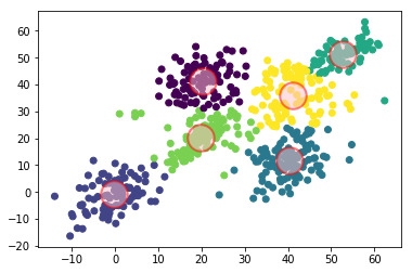
アノテーションのサポート (annotationQueryの実装)
Grafanaには、ユーザがグラフの中に注意を喚起するラベル(またはラベルの範囲)を
設定する機能がある。
ユーザが自力で書くだけでなく、プラグインがアノテーションを提供することもできる。
simpod-json-datasourceプラグインは、アノテーションを提供する機能を有する。
公式の説明はこちら。
例えば下図で薄く赤くなっている部分が プラグインによるアノテーション。
実装方法は以下。
- アノテーションサポートを有効にする
- annotationQueryインターフェースを実装する
- アノテーションイベントを作成する
アノテーションサポートを有効にするためには、
plugin.json に以下を追加する。
{
\"annotations\": true
}
simpod-json-datasourceプラグインのannotationQueryの実装は以下。
annotationQuery(
options: AnnotationQueryRequest
): Promise {
const query = getTemplateSrv().replace(options.annotation.query, {}, \'glob\');
const annotationQuery = {
annotation: {
query,
name: options.annotation.name,
datasource: options.annotation.datasource,
enable: options.annotation.enable,
iconColor: options.annotation.iconColor,
},
range: options.range,
rangeRaw: options.rangeRaw,
variables: this.getVariables(),
};
return this.doRequest({
url: `${this.url}/annotations`,
method: \'POST\',
data: annotationQuery,
}).then((result: any) => {
return result.data;
});
}
プラグインからURLにPOSTのBODYで渡ってくるデータは以下。
{
\"annotation\": {
\"query\": \"hogehoge\",
\"name\": \"hoge\",
\"datasource\": \"JSON-ikuty\",
\"enable\": true,
\"iconColor\": \"rgba(255, 96, 96, 1)\"
},
\"range\": {
\"from\": \"2015-12-22T03:16:16.275Z\",
\"to\": \"2015-12-22T03:16:18.102Z\",
\"raw\": {
\"from\": \"2015-12-22T03:16:16.275Z\",
\"to\": \"2015-12-22T03:16:18.102Z\"
}
},
\"rangeRaw\": {
\"from\": \"2015-12-22T03:16:16.275Z\",
\"to\": \"2015-12-22T03:16:18.102Z\"
},
\"variables\": {
\"variable1\": {
\"text\": [
\"All\"
],
\"value\": [
\"upper_25\",
\"upper_50\",
\"upper_75\",
\"upper_90\",
\"upper_105\"
]
}
}
}
これに対して以下の応答を返すとイメージのようになる。
以下はAnnotationEvent型と型が一致している。
isRegionがtrueの場合、timeEndを付与することでアノテーションが領域になる。
isRegionがfalseの場合、timeEndは不要。
tagsにタグ一覧を付与できる。
[
{
\"text\": \"text shown in body\",
\"title\": \"Annotation Title\",
\"isRegion\": true,
\"time\": \"1450754170000\",
\"timeEnd\": \"1450754180000\",
\"tags\": [
\"tag1\"
]
}
]